How to distribute a Tensorflow model as a JavaScript web app

We will build a handwriting-to-text feature for a website or app using Tensorflow.js (demo link). This means in practice that a user will draw a character (using the fingers on a phone or the mouse on a computer), the image will then be passed into our model which predicts a character, directly in the browser without having to do round trips via the server.

Although it is technically possible to also train the model in JS using Tensorflow.js, this is usually not the most suitable solution due to the fact that the client (the browser) will perform the computations, which is usually is run on a laptop or a mobile phone with limited hardware in terms of computational power. Therefore the training will first be performed using the Python library Tensorflow which supports model training on a larger GPU which is available through Google Colab for quicker training sessions. Once the training is done we export the model using another Python library tensorflowjs converter, so that it can be loaded in a web browser where the predictions will be made.

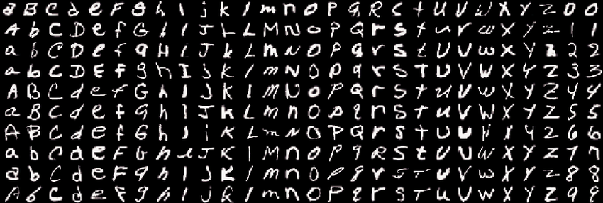
As is often the case with ML, in order to produce a model with a decent accuracy, we need a sufficiently large data set to train the model on. We decided to go with a data set EMNIST, a super set if you will to the popular MNIST data set. EMNIST contains not only the characters 0-9 like it's cousin MNIST, but also the latin ascii characters a-z and A-Z, which makes it applicable to our problem.

The EMNIST dataset has multiple different categorizations depending on your choice, see the histogram below from the original paper for a visual comparison.

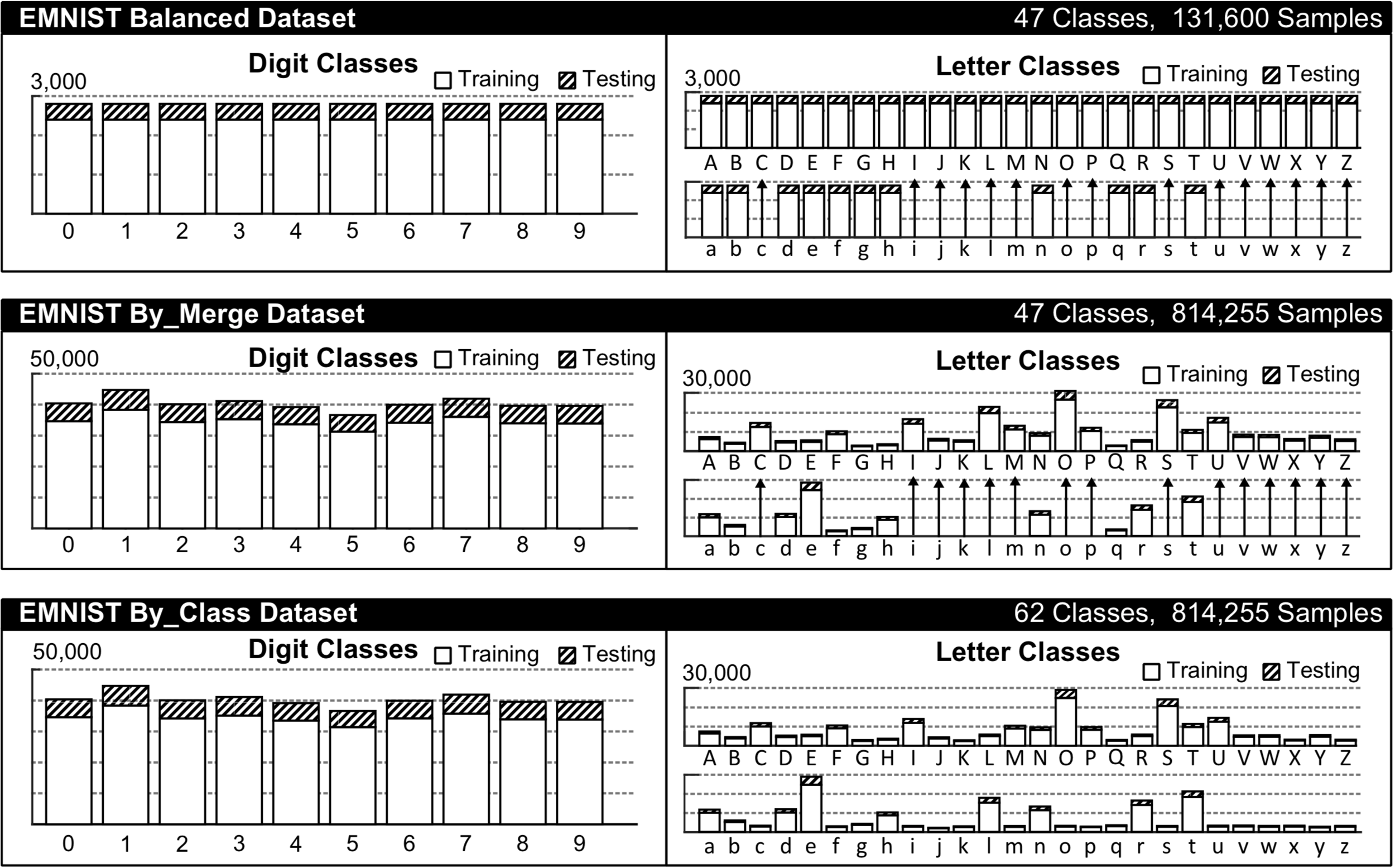
We're going to choose the categorization called By_Class for this task, since we want to be able to predict both upper and lower case characters as well as digits. Although the data set is fairly large (62 classes with 814 255 samples in total, where 697 932 of them are for training) it is quite heavily imbalanced, which can often lead to unwanted biases in the ML model towards the majority classes. However, for the purposes of this article, which is rather focused on how to get a model deployed in JS we'll have to live with these potential biases for now and move on to the training.

Downloading and extracting the EMNIST data set to your machine is done as follows:

Note that the leading "!" is only necessary if you run it in a Jupyter environment.

Loading your data set into memory for further processing is easily done with the help of the python library called python-mnist. To install run pip install python-mnist. Then we're ready to import the python packages and load the data set:

As you can see, we have 697 932 training samples and 116 323 test samples, which are 784-dimensional vectors. We want to transform these into 28281 3-dimensional tensors and normalize them (which can speed up training).

That looks better. Now for the target vectors. As you can see above, there are two lists of 697 932 and 116 323 scalars representing the different classes. Since the model we're creating is going to perform a multi class classification task, we need to one-hot encode these values (also known as dummy variables):

For image classification tasks such as this one Convolutional Neural Networks (CNNs) are often the best performing models, thus we will use one here.

Since the model will be deployed and used on the web, the smaller file size the better, therefore we restrict the amount layers in the model. This kind of model size- vs. accuracy-trade off has to be considered carefully. In our tests, we found that the following settings gave us a good enough performance while keeping the model under 0.5 MB when converted.

For a graphical overview our model, there's a nice helper method (click on the image below to enlarge it):

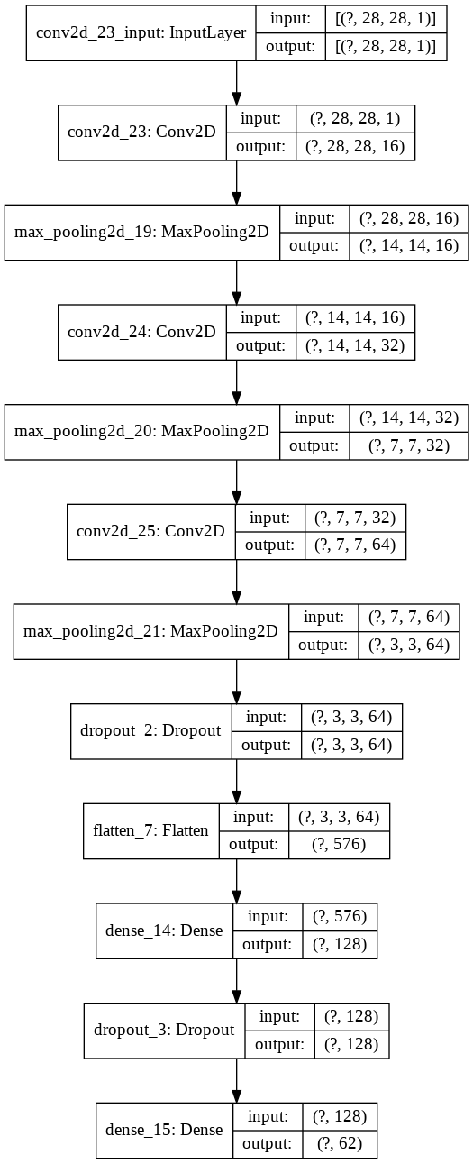
The model is now ready to be trained. The tf.keras.callbacks.EarlyStopping function is a convenient way of letting the model train until an optimum is found, meaning when the validation loss function won't go lower for let's say 10 epochs. The validation is performed on the test data set.

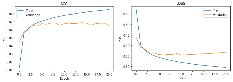
Looking at the results, we see that the accuracy of the predictions on the test set reaches a maximum of about 86% after 10 epochs. Not really a fantastic score, but still acceptable.

Let's get some better insights into where the model fails to predict the right values. This is easily visible with the help of a so called confusion matrix. We evaluate predictions on our test data set in relation with their true values, which looks something like the image below.

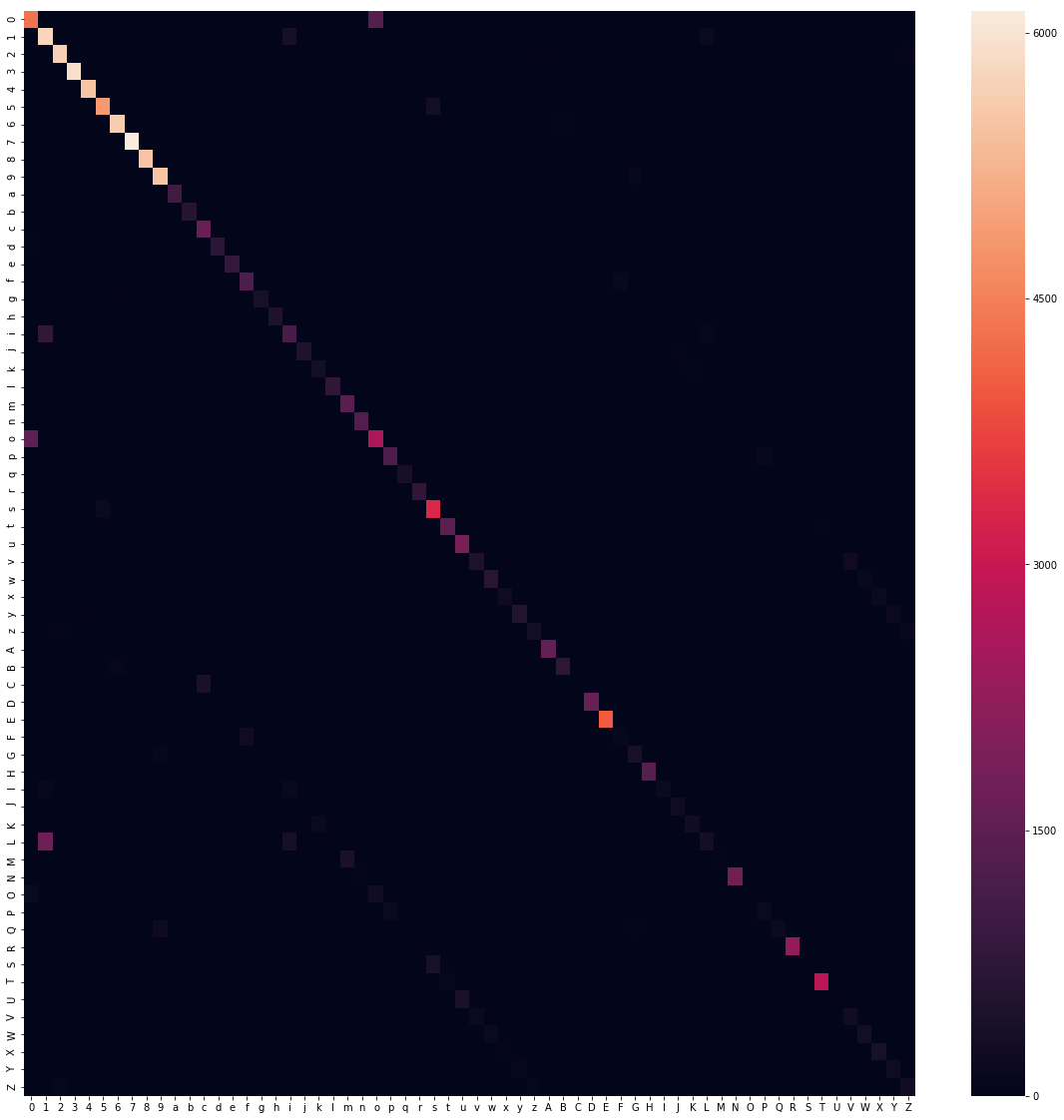
Exporting the model is made easy with the help of the Python library tensorflowjs. The tensorflowjs_converter terminal command produces two files: the model.json file which describes the model's setup, topology, type of layers, inputs and outputs, etc. The other .bin file is a binary file containing all the trained weights. We simply store our keras model to disk, and then convert it into the right format.

Now, we're ready to start producing the web app that will use this model for handwriting character recognition.

Before we begin with coding, let's discuss requirements of the web app for a second. There are two major components in this app: a hand drawing component and model prediction component. The latter is taken care of by tensorflow.js, we just need to prepare the image from the canvas before passing it to our model. For drawing, there are tons of great JS libraries out there, so let's not reinvent the wheel here. Upon some investigation, fabric.js seems to have the all capabilities we need as it supports free hand drawing to canvas as well as a bunch of helper functions that will come in handy later. In order to keep things tidy, we will create two classes Handwriting and Model, which wraps all methods and variables concerning each task respectively.

Let's first look at the drawing component. We would like to have a large full screen canvas, where the user can draw where ever he/she wants. Once the user has drawn something, we want to capture only the area where something is drawn, instead of scaling down the entire canvas to 28281 (our model's input size), which would likely obscure the actual drawing heavily.

First, let's set up our html document and load the necessary JS dependencies.

And voilà, now we can paint freely on the canvas. Next we would like to extract the pixel data created by the user, but nothing else. No unnecessary blank canvas outside the actual drawing. The fabric.Group method groups our collection of strokes on the canvas into a group which conveniently gives us values such as total width, height, x- and y-offset.

Note that we have to scale all factors by scale = window.devicePixelRatio to account for high resolution screens where 1 physical pixel doesn't always represent 1 virtual pixel. Later we'll show how to and when to call the method captureDrawing() but in the most minimal form, this is all we need from the Handwriting class, so let's move over to our Model class and see how we can get a prediction on what was just drawn.

In our class Model constructor, we need to first load our exported TensorFlow model and weights and assign it to a class variable. This is done as follows:

Here, tf.loadLayersModel() returns a Promise which, once resolved, returns our model object which is ready to do predictions.

However, before we can go ahead and try our first prediction in JS, we need to prepare the the image a little bit. The image will most certainly not have the right dimensions when passed over from the Handwriting class. Therefore we create a preprocessImage() method, which ensures that it matches the requirement of the model.

Note that the tf.tidy() function helps cleaning up all temporary tensors once executed to avoid memory leaks.

Ok, time for our prediction. We create a method that takes the pixel data from the Handwriting class, preprocesses, makes a prediction, and then retrieves the most probable character.

Note that operations on the tensors aren't directly accessible to us in the JS runtime. They might be run on the GPU and to avoid unnecessary traffic between the CPU and the GPU, you need to call .dataSync() explicitly to retrieve the value.

That's it, now we have everything needed to make a prediction. Simply run:

Our job is not really done here though. The web app is hardly interactive enough to be useful. We want to clear the canvas once the character has been obtained and predicted, so that we're ready for the next prediction. Therefore we need to set a timer after the user has stopped painting. This timer is cancelled each time the user touches the canvas again, but as soon as we register a certain amount of time without any interaction, we capture what's drawn (after some experimentation, 800 ms on desktop and 400 ms on touch devices seem like a decent choice). Let's add the following code to the Handwriting class.

The above mentioned functions are all you need to build an interactive web app that predicts hand written characters from the user. However, a lot of additional features could be wished for in order to make this a nice app to interact with such as: canvas auto-resizing with the browser window, displaying the output of the model on the website, variable stroke width, clear/submit button, pre-warmup of the model to improve latency, etc. Unfortunately this would mean that this already lengthy article would become even longer.

If you want to have a look at the source code of the end result, check out our Github repository to download the project in its entirety. For a live demo look at the iframe below or click here for a full screen version of the app.