What is Reinforcement Learning? (Part 1)

MDP

The mathematical object at the center of RL is the Markov Decision Process (MDP). An MDP is defined as follows:

A MDP is a 4-tuple $$(S, A, R, P)$$, where $$S$$ is the set of states, $$A$$ the set of actions, $$R: S\times S \times A \rightarrow \mathbb{R}$$ a reward function and $$P: S \times S \times A \rightarrow \left[ 0, 1\right] $$ the conditional transition probability.

Reinforcement learning means that an agent, which could be a chatbot, a self-driving car etc., interacts with the MDP in that it finds itself in a state $$s \in S$$, where it has to choose an action $$a \in A$$. After applying $$a$$ to the environment, the agent finds itself in the state $$s' \in S$$ via the transition probability $$s' \sim P(\cdot | s, a)$$. For this move the agent is rewarded or punished with $$R(s',s,a)$$. A well-known real-world example of this type of learning is operant or instrumental conditioning in dog training.

The agent's behavior is represented by the policy $$\pi: A \times S \rightarrow \left[ 0,1 \right]$$, which is the probability of choosing action $$a$$ when in state $$s$$. The goal of the agent is to learn an optimal policy $$\pi^{\prime}$$ such that the expected cumulative discounted reward is maximized, i.e.

[Loss]

where $$r_t := R(s_{t+1}, s_t, a_t)$$ is the reward received at time step $$t$$ and $$s_{t+1} \sim P(\cdot | s_t, a_t)$$. $$T$$ is the number of steps taken in the MDP and often we have $$T \rightarrow \infty$$.  $$\gamma$$ is just a discount factor satisfying $$0\leq \gamma \leq 1$$.

Generally, $$P$$ might be unknown to the agent (model-free RL), but the MDP can be sampled and the optimization problem [Loss] can be solved with Monte Carlo simulations.

Model-free RL algorithms can be further categorized by how $$\pi$$ is treated. There is the category where $$\pi$$ is modeled directly, which is known as policy-based RL. On the other hand, there is value-based RL, which is what we will discuss here. The name already gives the idea that value-based RL methods rely on some value function. Usually, the value function of interest is the so-called $$Q$$-function. The $$Q$$-function $$Q(s, a)$$ maps state-action pairs to the expected reward, if the agent started out in state $$s$$ and took action $$a$$, i.e.

[DefQfunction]

with $$\pi$$ being a greedy policy with respect to the Q-function. A greedy policy is a policy that in any state $$s$$ always chooses the action $$a = {\mathrm{argmax}}_{a'} Q(s, a')$$. As a short-hand, one can think of the Q-function $$Q(s, a)$$ to measure how "good" it would be to take action $$a$$ in state $$s$$ and act greedily in all subsequent states.

This poses the question of how $$Q(s, a)$$ can be learned from sampling the MDP. In the MDP at every timestep $$t$$, the agent observes an experience $$(s_t, a_t, s_{t+1}, r_t)$$, sometimes also called a transition. In the beginning we can guess the Q-function randomly and start simulating the MDP. After each transition we perform the update step

[QLearningUpdate]

with $$\alpha$$ as the learning rate. If $$s_{t+1}$$ is a terminal state of the MDP, the update step looks like

[QLearningUpdateTerminal]

[QLearningUpdate] can be rewritten as

[QLearningUpdate2]

The bracketed term on the right hand side is called the temporal difference (TD-)error, hence this type of Q-learning is called temporal difference learning.

Q-Learning works by sampling the MDP and updating the Q-function according to the gathered experiences. A property of the MDP is that decisions made earlier have an influence on the states that the agent will be visiting throughout the run of the MDP, which in turn influences the experiences that are gathered and the Q-function updates that are made.

Consider an agent that only takes actions that are optimal according to its current Q-function. The agent progresses deep into the MDP and gathers valuable experiences for later stages. That is to say, the agent exploits its current knowledge to gather experiences that are valuable. However, the current Q-function might be off and lead to a suboptimal behavior. It could be advantageous for the agent to explore new ways to go, e.g. by randomly guessing a few actions. This will lead to random experiences and might help discover new, potentially better strategies. This dilemma is known as the exploration-exploitation trade-off.

There are a few ways to engage with this trade-off. The most well-known approach would be to use an $$\epsilon$$-greedy policy. $$\epsilon$$-greedy means that the agent in state $$s$$ picks the greedy action $$a = {\mathrm{argmax}}_{a'} Q(s, a')$$ with a probability of $$1-\epsilon$$ for some $$\epsilon \in [0,1]$$ and uniformly samples $$a$$ at random otherwise. Usually $$\epsilon = 1$$ is chosen in the beginning of training and gets decreased over training time by some decay schedule, e.g. $$\epsilon(t) = k^{-t}$$ for some decay parameter $$k < 1$$.

So far we did not make any assumptions about the implementation of the Q-function. In principle, it could be a simple table. However, this is technically infeasible for many applications, as the state space $$S$$ would be too large. If $$S$$ is continuous, we would furthermore need to introduce a discretization, which is generally quite lossy. A real breakthrough in the field of RL was achieved by DeepMind in 2013 with the introduction of Deep Q-Learning (DQN).

In DQN the Q-function is approximated by a deep neural network (DNN), which takes $$s$$ as inputs and outputs a vector where the $$a$$-th element is the Q-value for the action $$a$$, i.e. $$Q_a(s|\theta)$$, where $$\theta$$ is the set of parameters of the neural network. In order to use a DNN as an approximator of the Q-function, the update rules [QLearningUpdate] and [QLearningUpdateTerminal] need to be re-formulated such that they can be performed using gradient descent. Consider

[DQNUpdate]

with the loss function

[DQNLoss1]

if $$s_{t+1}$$ is a non-terminal state of the MDP and

[DQNLoss1Terminal]

if $$s_{t+1}$$ is terminal. Note how in the target value $$r_t + \gamma \max_{a'} Q_{a'}(s_{t+1}|\theta')$$ a different set of parameters $$\theta'$$ is used. This is because gradient descent should only update the Q-network towards the target value and keep the target value fixed. In practice this can be done by computing the target value first and consider it constant in the loss function.

Also it has been shown that training is more stable, if $$\theta'$$ is not updated after every gradient descent step, but only with a certain period, e.g. every 10th, 100th or 1000th update step. This way, disturbing feedback loops of noise are prevented. To implement the delayed updating of $$\theta'$$, a secondary model with parameters $$\theta'$$ is maintained, where $$\theta'$$ only gets updated according to the update period. This secondary model is called the target network or target model.

Double Deep Q-Learning

One problem with the TD error [DQNLoss1] is that the maximum over $$a'$$ is used in the target value. This causes the Q-function to over-estimate the Q-values. In order to mitigate this effect, Double Deep Q-Learning was introduced. In Double Deep Q-Learning the target value requires two different networks, one for choosing the optimal action at the next state and one for the Q-value of said action. In practice, the action is chosen with the primary model, while the Q-value is taken from the target model. The loss function now looks like

[DQNLoss2]

with

[DQNLoss3]

Note the different Q-function parameters $$\theta$$ and $$\theta'$$ in [DQNLoss2] and [DQNLoss3]. This way minimizing the TD error does not necessarily move the Q-function towards the maximal value of the target and thus helps preventing over-estimation of the Q-function.

Experience Replay Buffer

The following problem can occur when using an DNN as the Q-function approximator: When updating the model parameters, not only the Q-value of the particular training data point used to compute the TD error is changed. In fact, the Q-values for many action-state pairs will change in an uncontrolled manner. This can cause what is known as catastrophic forgetting. Mnih 2015 introduced a technique called Experience Replay Buffer (RB) to mitigate this effect.

The transition $$(s_t, a_t, s_{t+1}, r_t)$$ is stored in the RB. Once the Q-function approximator's parameters are updated, the DNN is not trained on this single transition, but on a mini-batch of size $$M$$ of randomly sampled transitions from the RB. Hence, transitions from the past are used as well when updating the model parameters. This helps to prevent catastrophic forgetting.

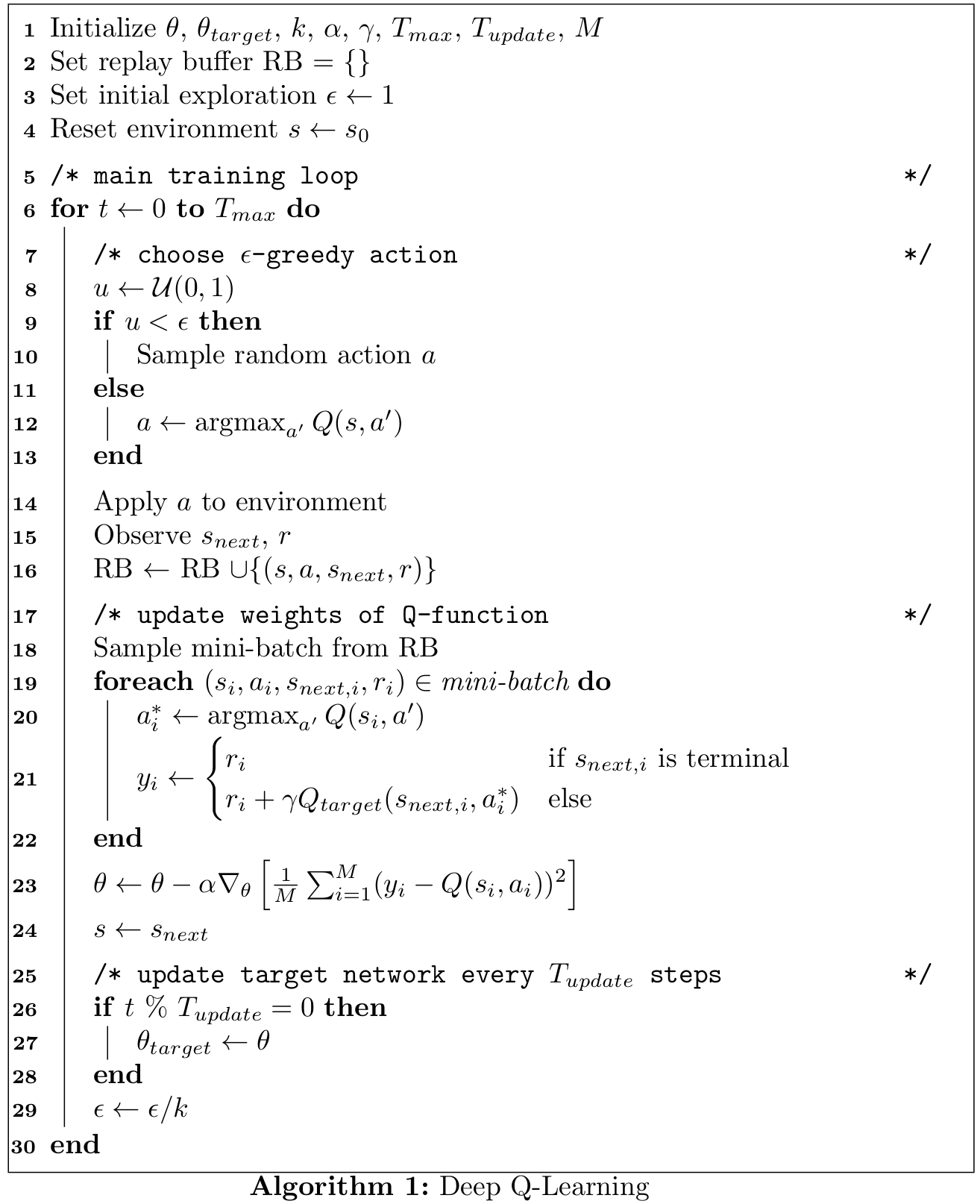
The algorithm

Putting all the discussed concepts together, we end up with the following algorithm. $$\theta$$ and $$\theta_{target}$$ parameterize the primary and target models respectively, $$k$$ is the $$\epsilon$$-decay schedule, $$\alpha$$ the learning rate, $$\gamma$$ the discount factor for the discounted reward, $$T_{max}$$ the maximum number of steps to run, $$T_{update}$$ the period of target model updates and $$M$$ the batch size to sample from the RB.

Let's discuss a small example. We use an environment from the OpenAI Gym library. OpenAI Gym is a Python library that implements various little games to play with. We choose the LunarLander environment. The goal is to land the lunar module on a landing pad without crashing it. The location of the module is described by the coordinates $$x$$ and $$y$$, while the origin of this coordinate system is placed in the center of the landing pad. At the beginning of each episode, the module starts above the landing pad with a randomly chosen but small velocity. The lunar module has two legs, which need to touch the ground in order to land. The legs are attached to the module via springs. If the springs get so compressed that both or one of the legs touches the module, the episode is finished. This way, the agent is supposed to learn to fly and carefully land the module, rather than crashing it into the ground.

For control the module has three engines: the main engine pointed downwards and two less powerful side engines. The firing of the engines is modeled by small red spheres being ejected into the directions of the respective engine with some small random disturbance added to their momentum. The repulsion from ejecting the spheres propels the lunar module. The main engine is much more powerful than the side engines, because the main engine is supposed to be used for levitation, while the side engines are for balancing the module.

The dimension of the state space $$\dim(S) = 8$$, where each state $$s$$ is given by

where $$x$$ and $$y$$ are the coordinates of the center of gravity of the module, $$\dot{x}$$ and $$\dot{y}$$ are the respective velocities, the angle $$\phi$$ describes the module's pitch and $$\dot{\phi}$$ is the respective angular velocity. $$C_r$$ and $$C_l$$ are boolean variables and equal to 1 if the right or left leg touch ground and 0 otherwise. The dimension of the action space $$\dim(A) = 4$$, where the agent can choose to do nothing ($$a_1$$), fire the right side engine ($$a_2$$), fire the main engine ($$a_3$$) or fire the left side engine ($$a_4$$).

The reward at time step $$t$$ is issued according to

[LunarLanderReward]

where $$F_\text{main}$$ and $$F_\text{side}$$ are boolean variables indicating if the main or one of the side engines was fired. The subscripts $$t$$ and $$t-1$$ indicate the time steps. The reward [LunarLanderReward] incentivizes the agent to stir the lunar lander towards the landing pad at the origin, which is described by the first two terms in the brackets. Furthermore, it is rewarded to keep the velocities limited, as the third and forth term rewards flying slower than in the previous time step. It is also rewarded to decrease the module's pitch. The terms $$+ 10(C_{rt}-C_{rt-1}) + 10(C_{lt}-C_{lt-1})$$ reward ground contact for each leg and punish, if the legs break ground contact. The last two terms punish the usage of the engines. This incentivizes the agent to fly with less engine use, although in this simulated environment fuel is not limited. As mentioned above the episode ends, if the module crashes onto the ground such that the legs touch the module, in which case a reward of -100 is issued instead of [LunarLanderReward]. If the module come to a halt without crashing, the episode ends as well and a reward of 100 is issued to the agent.

For more detail, consult the documentation or the original source code.

In the following animation we can see how the agent slowly gets better at landing the module over time.

While in the beginning the lander just hopelessly crashes into the ground, the agent learns to hover the craft after about 500 episodes of training. After that the landings are very shaky, but over time they become more and more secure. The performance could probably still improve with more training.

Deep Q-Learning is a very basic approach to RL, but it allows to highlight some of the challenges that need to be over-come to find good solutions to RL problems. There are a few problems that need to be addressed.

Continuous Action Spaces

So far, we tacitly made the assumption, that the action space $$A$$ is discrete, or at least can be discretized sufficiently well. Oftentimes this is not possible and a way to deal with continuous $$A$$ is needed. The basic algorithm to use DNNs for continuous $$S$$ and $$A$$ is Deep Deterministic Policy Gradient (DDPG).

Efficient Exploration

While $$\epsilon$$-greedy is the most well known solution to the exploration-exploitation trade-off, there is active research on other methods that have been shown to be more efficient in some cases. Most notably, people are trying to use Bayesian methods and combine them with Deep Learning techniques.

Multi-agent RL

Above we exclusively discussed RL algorithms that use a single agent that engages with the environment. For many tasks it is necessary to have several independent agents that coordinate their efforts to reach a common goal or that compete for resources to reach diverging goals. This is the field of Multi-Agent RL (MARL). MARL is actively researched and quite a few impressive advances have been made in recent years. MARL will be discussed in more detail in the next post of this series.

Some drawbacks

RL is one of the most promising approaches to what some might consider artificial "intelligence". However, there is a few issues. First, RL algorithms depend strongly on the ability to sample the process they are supposed to control. The agent needs to learn from trial and error by repeating the scenario over and over again, usually thousands of times. This is infeasible in the real world, hence a simulation environment needs to be provided. This in turn requires a lot of effort, as the simulation needs to capture every relevant aspect of the problem at hand.

The second problem arises in particular if DNNs are used as Q-function approximators. DNNs are notorious "black boxes". Their inner logic is oftentimes not well understood and hence extra caution needs to be given to security aspects and how the agent learns to reason about its environment. There have been examples of RL-agents seemingly being able to solve a task perfectly and later it turned out that they were deciding based on artifacts of the simulation. Once confronted with a slightly different scenario, the agents, surprisingly to their developers, started failing.

Another issue is the reward function. It needs to be designed in such a way that it incentivizes the desired behavior and punishes unwanted aspects. Otherwise the agent might figure out strategies that are numerically optimal, but neglect the true goal.

I hope you were able to get a high-level overview of the topic of Reinforcement Learning and some of its challenges. In the next part we will discuss in more detail the state-of-the-art of MARL.