Semantic segmentation of satellite images
Nelson Martins (PhD)

This post presents some key learnings from our project on identifying roofs on satellite images. Our aim was to develop a planing tool for the placement of solar panels on roofs. For this purpose we set up a machine learning model that accurately partitions those images into different types of roof parts and background. We learned that the UNet model with dice loss enforced with a pixel weighting strategy outperforms cross entropy based loss functions by a significant margin in semantic segmentation of satellite images.
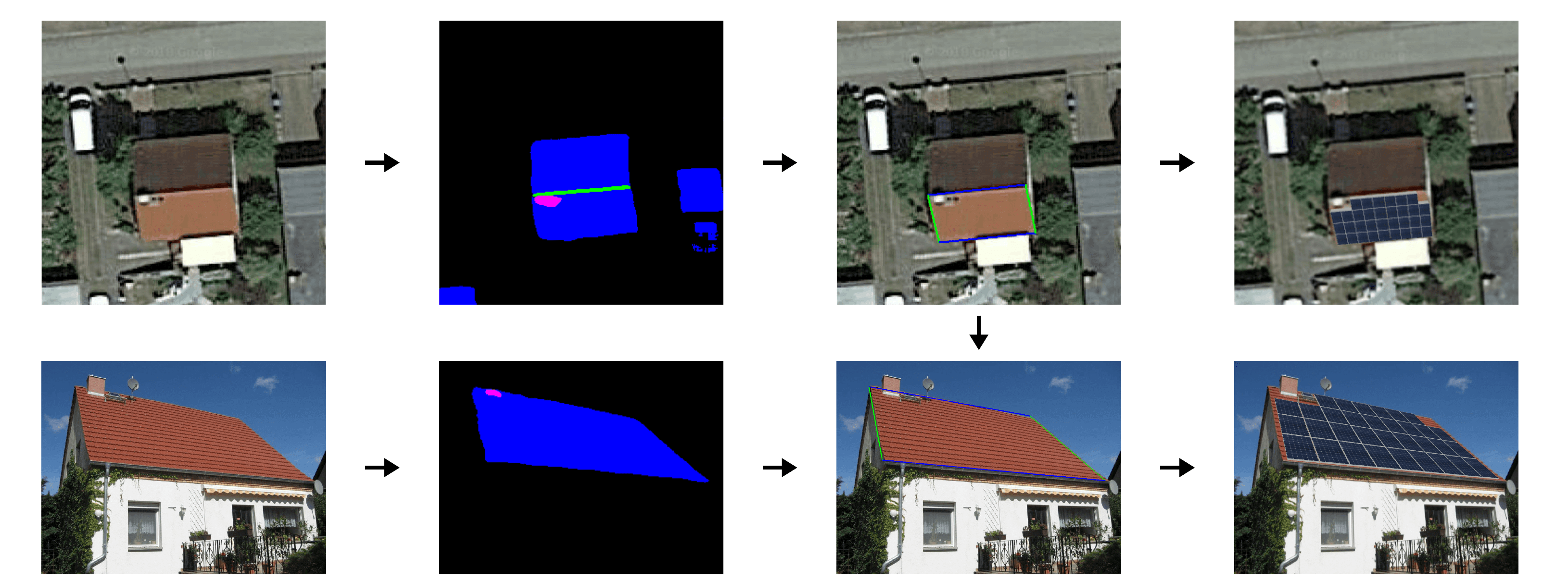
The following idealized pipeline illustrates the functionality of the planning tool:
Satellite Image Segmentation
Dataset
To achieve the proposed goal, we created a database with satellite images and the respective roof labels. The Google Maps API was used to gather a total of 1500 unique images from houses spread across Germany. The API accepts as input a value of latitude and longitude that identifies a specific region on the globe and a set of parameters to select the desired characteristics of the returned image. We chose parameters such that the obtained images had the best quality possible and most houses could be captured with a considerable margin in a single shot:
Image dimensions (RGB) |
Scale |
Zoom level |
Pixel size (m) |
Image size (m) |
|
Value |
400x400x3 |
1 |
20 (max) |
0.086 - 0.102 |
34x34 - 41x41 |
The pixel size is variable along the latitude and its value can be calculated as follows:
Here are some examples of the database images and their respective labels:
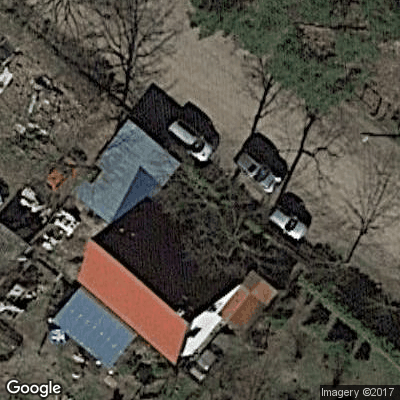


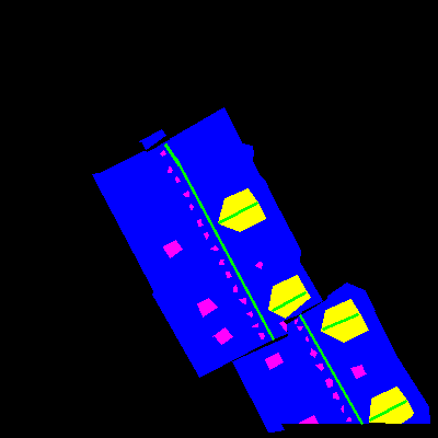
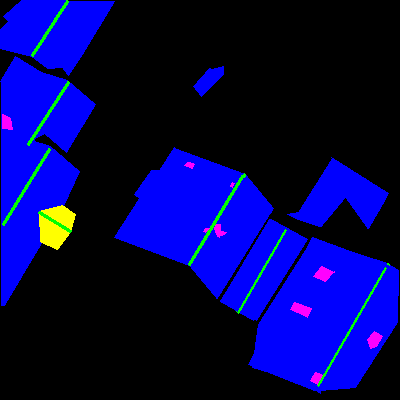
The labels are the roof (blue), obstacles (magenta), ridges (green) and dormers (yellow). The first is used to identify the area where solar panels can be placed; the second identifies areas where solar panels cannot be placed, such as antennas, chimneys, skylights; the ridges are used to separate roof sides and identify discontinuities on them; the dormers are a special case where people would only rarely want to place panels.
For a better understanding of the problem, we also present some data statistics based on these 1500 images:
Roof |
Ridge |
Obstacles |
Dormers |
Background |
|
Pixel ratio |
17.74% |
0.70% |
0.70% |
0.92% |
79.93% |
Image ratio |
100.00% |
99.41% |
98.50% |
48.99% |
100.00% |
From this table we learn that:
Most images have roofs, background, ridges and obstacles
Most pixels belong to the roof or background
Very few pixels belong to the ridges, obstacles and dormers
Dormers are found in around half of the images
In short: high class imbalance!
The UNet Model
The problem at hand falls into a semantic segmentation problem with high class unbalancement. One of the most successful deep learning models for image segmentation problems is the UNet Model:
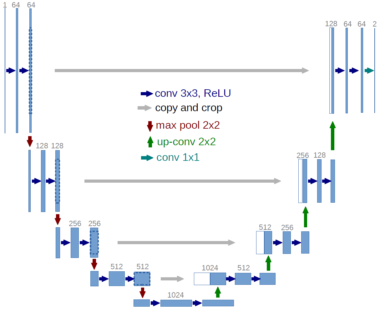
The UNet is a convolutional neural network (CNN) was first proposed for the automatic segmentation of microscopy cell images, but it is applicable to any segmentation problem. It is composed of an encoder followed by a decoder. The encoder is responsible for capturing different features at different scales and the decoder uses those features to construct the final segmentation map. In the UNet model, the encoder and the decoder are symmetric and connected with skip layers on every scale. These skip layers allow the reuse of feature maps from every scale on the decoder, which in practice results in more details being added to the segmentation. The following image illustrates the effect of skip layers on the segmentation results (FCN-32: no skip layers, FCN-16: one skip layer, FCN-8: two skip layers).
Image source: http://deeplearning.net/tutorial/fcn_2D_segm.html
Original work: https://people.eecs.berkeley.edu/~jonlong/long_shelhamer_fcn.pdf

Tests and tricks
Our first focus was on the creation of a stable pipeline. To do so, we started by splitting the data randomly:
Train set |
Validation set |
Test set |
|
Size |
1100 |
200 |
300 |
Next, we implemented the UNet, using the Keras API (a Python deep learning library running on top of TensorFlow), and made some adjustments:
Added batch normalization after all Conv2D layers
Conv2D activation changed to selu
Batch normalization is known for improving the convergence process and speed because it prevents the tensor values from overshooting. This also helps to keep the network weight under control since the feature values are always kept on the same order of magnitude.
The scaled exponential linear unit (selu) was proposed by Klambauer et al. as a self normalizing layer that extends and improves the commonly used ReLU activation:
The authors claim that the main advantage of this activation is that it preserves the mean and variance of the previous layers. Moreover, it helps prevent the Dying ReLU problem (and therefore vanishing gradient problems) since its derivative is different from zero for negative values. This work was followed by others that have shown an improvement on the trainings and results. Our preliminary tests confirmed those findings and so we decided to use it.
We also added data augmentation:
flips (up-down, left-right)
rotations (+/- 20º)
intensity scaling
Gaussian noise
Finally, the training hyper-parameters were obtained empirically using greedy optimization:
learning rate: 0.001
batch size: 8
activation: sigmoid
loss: dice + pixel weighting
optimizer: Adamax
learning rate scheduler: 50% drop after 20 epochs without improvement
All of these parameters played an important role in the training process, but the right choice of the loss function turned out to be crucial.
Loss functions
We tested the weighted class categorical cross entropy (wcce) and the dice loss functions.
Weighted class categorical cross entropy:
For an image with $$ d1 \times d2 $$ pixels and $$ K $$ classes the weighted class categorical cross entropy is defined as
where
The wcce loss function enforces that the model should output a probability value close to 1 for positive classes. In addition, each class has a weight $$ w_k $$ associated to control their importance. The class weight was set so that the detection of the ridge, obstacles and dormers is enforced:
Roof |
Ridge |
Obstacles |
Dormers |
Background |
0.2 |
0.3 |
0.25 |
0.25 |
0.05 |
Dice loss:
In the same situation as above, the dice loss is defined as
where
are matrices containing the predictions for all pixels with respect to only class $$ k $$, respectively the ground truth and
i.e. the element-wise product.
The dice loss is a continuous approximation of the well known dice coefficient. In our case, we calculated the dice loss for each class and averaged the results over all classes. This way, we are able to naturally take into account the class imbalance without adding a class weighting.
With these two loss functions we were able to achieve satisfactory results, but we found out that by penalizing the most frequent class (background) we were failing to classify some very important pixels: the ones that belong to the background between very close roofs. Because of that, we decided to follow the proposal of Olaf Ronneberger, et al. and add a pixel weighting component. This way we can enforce that some specific regions on the image are more important than others.
Pixel weighting:
where $$ c_1 $$ is the distance to the border of the nearest and $$ c_2 $$ to the border of the second nearest roof.
The following images illustrate how the pixel weighting emphasizes regions between adjacent roofs:

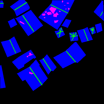
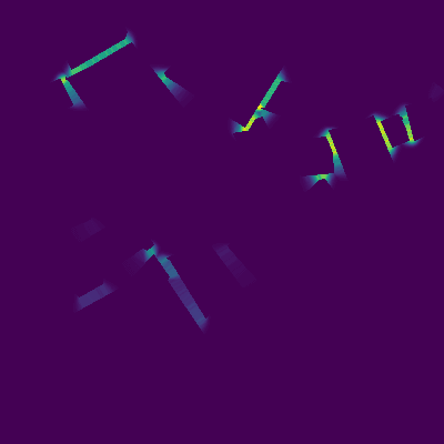

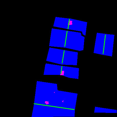

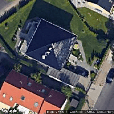


Pixel weighting was added to the wcce and dice loss as follows:
Class and pixel weighted categorical cross entropy:
Pixel weighted dice loss:
where $$ \text{wmse} $$ is the weighted pixel mean squared error:
With this strategy we can control the segmentation results on both the class and pixel level by tuning the loss function as desired. Next we present some of the obtained results.
Results
These are the plots of the mean dice coefficient obtained during training for the described loss functions:

The wcce leads to better results on the training set but worse on the validation, which indicates that it does not generalize as well as the dice loss. The pixel weighting pw did not change the train plots very much, but on the validation set sped up the convergence of the dice loss.
These are the results on the test set, class-wise:
wcce |
wcce + pw |
dice |
dice + pw |
|
Roof |
0.66 |
0.66 |
0.78 |
0.80 |
Ridge |
0.26 |
0.30 |
0.42 |
0.43 |
Obstacles |
0.34 |
0.38 |
0.52 |
0.51 |
Dormers |
0.27 |
0.50 |
0.64 |
0.68 |
Ground |
0.94 |
0.92 |
0.96 |
0.96 |
Attending to the results, it is clear that the dice loss outperformed the wcce and that the addition of the pixel weighting improved the results on both, making dice + pw the best combination of loss functions.
Finally, here are some of the resulting predicted segmentations (left: original satellite images, center: predictions by model with dice loss, right: predictions by model with weighted dice loss):

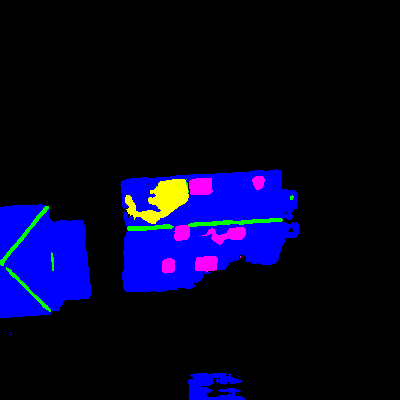
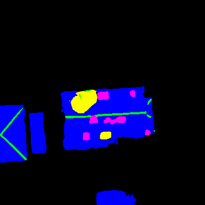


From the visual results it is possible to observe that the inclusion of the pixel weighting led to better margins and better roof separation in the case of very close roofs.
