Early Classification of Crop Fields through Satellite Image Time Series

To train any supervised model one needs to have labeled data. Our data is based on pairs of geometries describing the boundaries of fields and the name of the crop growing in said fields (the labels). Using the geometries we are able to extract the time series of pixels that are supposed to be mapped to the labels by the model from the raw satellite data (a time series of images). What we refer to as a parcel then is this bounded area defined by the geometry from which we have a collection of pixels that we want to obtain a prediction. Note that a pixel is a one-dimensional vector with a length equal to the number of channels of the image it was taken from.

It is also important to note that the images here are not exactly the same as the common images we are used to. In this context, an image is composed of many channels (depending on the source) as opposed to the common three channels (RGB).

The model’s inner workings can then be split into three parts:

• Pixel-Set Encoder: Where the model creates a time series of embeddings of the raw data, by encoding samples of pixels from one parcel.

• Temporal Attention Encoder: Where the previous time series are passed through a variation of Vaswani et al.’s Transformer that produces a single tensor as output.

• Classifier: Where the previous tensor is used to determine a crop class.

In the blog post “Classification of Crop fields through Satellite Image Time Series” we explain all these concepts in more detail.

The first change we applied was to use multi-modal data to classify the fields; Inspired by previous studies (Garnot et. al, Ofori-Ampofo et. al) we decided to include Sentinel-1 (SAR data, also known as radar data) alongside the Sentinel-2 (Optical and Infrared data). The reasoning behind using Sentinel-1 (S1) is that there are two limitations of Sentinel-2 (S2) that reduce its data availability:

• Cloud coverage: S2 collects data within an interval of the electromagnetic spectrum that cannot penetrate clouds. This means that if a cloud is present within the satellite's view, no data will be acquired from the ground below it.

• Daylight: S2 is designed to create images using Earth’s reflected sunlight. Thus it can only collect data if the patch it is flying over is illuminated by the sun.

S1 data, on the other hand, can be used to mitigate these missing data points, since it doesn’t suffer from either of these limitations. Not only does it have its own source of electromagnetic radiation, but also the type of radiation it produces (radio waves) can penetrate clouds and retrieve surface information that lies underneath them.

The difficulty with doing this now is that observations from either source are obtained at different points in time. The picture below illustrates the occurrences of data from both data sources for two different parcels over the course of a year. There we can see how the timestamps of the observations differ, not only between sources (S1 and S2) but also between observations of the same source on different parcels (A and B).

There are different ways one can fuse sequential data that doesn’t share the same temporal availability. They differ on when (and how) the data from the different sources are merged together. For our purposes, we decided to use Early fusion, as it was demonstrated by the authors of the previously mentioned papers to be the most memory efficient of the fusion models while also showing substantial gains in performance as compared to models using single sources.

Early fusion combines the sources’ data before it is fed to the model. Images from both S1 and S2 are usually interpolated so that the time series match in length. This creates two new time series that have data points at matching times. This way the fusion can be done at the channel level, that is, one can just stack all channels of the images that match in timestamp. Effectively this creates a new time series where each image is composed of channels from S1 and S2.

We also introduce some novelty to it by skipping the interpolation step (“temporal resampling” in the sketch from Garnot et al.) altogether by just padding the series of either source when a matching timewise observation is not available. This means that whenever there is an observation, for example from S1, that has no corresponding S2 observation, the fused series will include that S1 observation concatenated with a “missing data” value in place of the missing S2 data.

Finally, using this kind of model (a Transformer) solves the problem of having different parcels with completely different time series in terms of length and frequency of data. As mentioned before and in the previous blog post, one of the components of the model is the positional encoder. This component takes in, along with the pixels used for prediction, a list of the acquisition dates of the pixels. These essentially communicate to the model how these pixels are positioned in time. This gives the model a sort of extra dimension to compare time series; the model doesn’t have to be restricted to comparisons between data points with the same index and can perceive more complex relationships within and between time series.

The table below shows the results of evaluating the model with and without the fusion of sources. The model was trained and evaluated using data from the growing cycle of 2018. As seen in the table when using fused data there is an increase in the performance of the model as compared to using either singular source. This is due to the fact that now the model has access to some of the information that is missing due to the S2 data unavailability. It also means that in regions where cloud occlusion is a larger problem (there are even fewer available S2 images) the model is still expected to perform well.

The main objective of our project was to achieve a plausible classification of a parcel as soon as possible within its growing cycle. Again there are many ways one can go about achieving early classification:

• Same model, different times: This basically means that one trains a model for each of the time periods a prediction is needed on.

• Crop rotation patterns: The idea behind this concept is that certain crops tend to rotate in a predictable way, that is farmers plant these crops one after another following a recognizable pattern. By using a model that has been trained on data from many years the model is able to recognize these patterns and infer what is currently growing before it is even planted.

• Expertise-based model: Some researchers are able to also build models out of their expertise about the crops. They can use their knowledge about how the data “looks like” for a given crop at a given time to create a decision tree that arrives at a correct crop classification without having to train a model.

Our solution was to simply train a model on randomly masked time series: While training we augmented our data by randomly obscuring the data of each parcel’s time series after a number of days from its beginning. Doing this gives the model examples of what data would be available for a classification earlier in the growing cycle. This forces the model to not always rely on the full time series (from seeding to harvest), but rather find other patterns within the data in order to be able to make predictions. It also means that it can make sense of incomplete time series of data allowing it to generate early predictions. 

Below we can see a representation of this early classification technique with a graph that shows how the performance of the model grows (up to a point) with the amount of data available from the growing cycle.

Here we also show how the model performance changes with data availability in time, specifically for rapeseed and sugar beet. The areas shaded in green and yellow represent the periods of time when these crops are usually seeded and harvested, respectively. The colors of the lines have the same legend as the previous image.

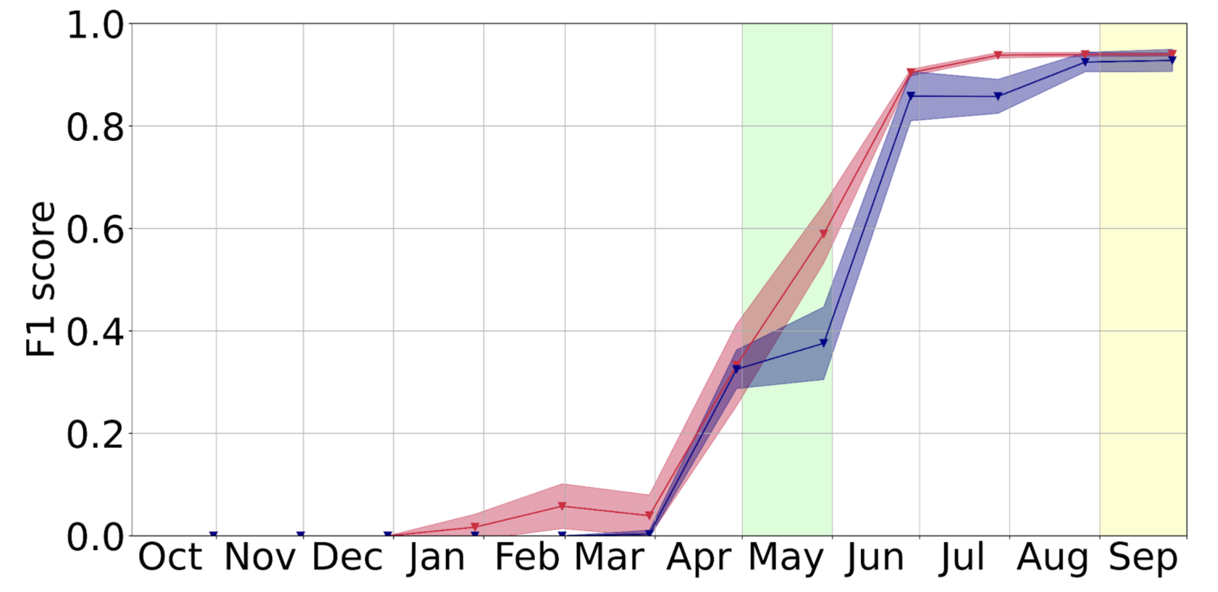
In the images above the graphs contain two lines, one corresponding to 2018 & 2019 and another corresponding to 2020. These indicate the F1 scores the model achieved when evaluated on a date from those years. The model was always trained with data from 2018 & 2019. Another important aspect is the bands around the lines. These represent the mean (the line) and the standard deviation of the scores obtained from evaluating different training instances of the model.

This article shows how the model in “Classification of Crop fields through Satellite Image Time Series” was altered in order to be able to use other data sources and to perform early classification. For more in depth explanations about how we achieved these results, we invite you to read our published paper about the subject called “Early Crop Classification via Multi-Modal Satellite Data Fusion and Temporal Attention”.